Plots in GAMLj

library(GAMLj3)

Obtaining a plot

GAMLj functions (gamlj_lm(),gamlj_glm(),gamlj_mixed() and gamlj_gmixed()) can produce plots including up to three variables. The plots portrait the model predicted values in the Y-axis. Using the functions, one can obtain the plots by using the following options:

plot_x the variable in the X-axis
plot_z the moderator variable, whose levels define the traces (separated lines)
plot_by the variable whose levels define the two-way interactions in multiple plots (separated plots)

Example

We use the iris R dataframe. Assume we want to plot the influence of Sepal.Width, Petal.Length and Petal.Width on Sepal.Length, and their interactions. We use gamlj_lm() to estimate the model and ask for the plots.

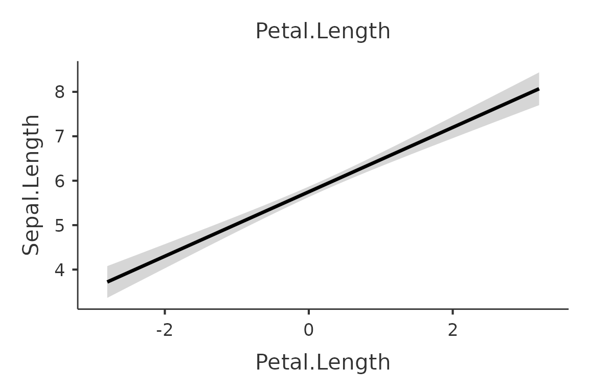
First we ask for the plot of the main effect of Sepal.Width. We use plot() without any option to extract the plot from the galmj results object.

mod<-gamlj_lm(formula=Sepal.Length~Sepal.Width*Petal.Length*Petal.Width, 
              data=iris,
              plot_x = "Sepal.Width"
              )

plot(mod)

To have additional plots, we can re-estimate the model using the options described above or using plot(). The function plot() accepts either a formula or character options. The formula is a right hand side formula specifying the X-axis variable and the (optional) moderators.

Examples are:

One-way plots

plot(mod,formula = ~Petal.Length)

Two-way plots

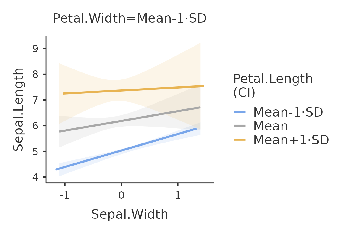
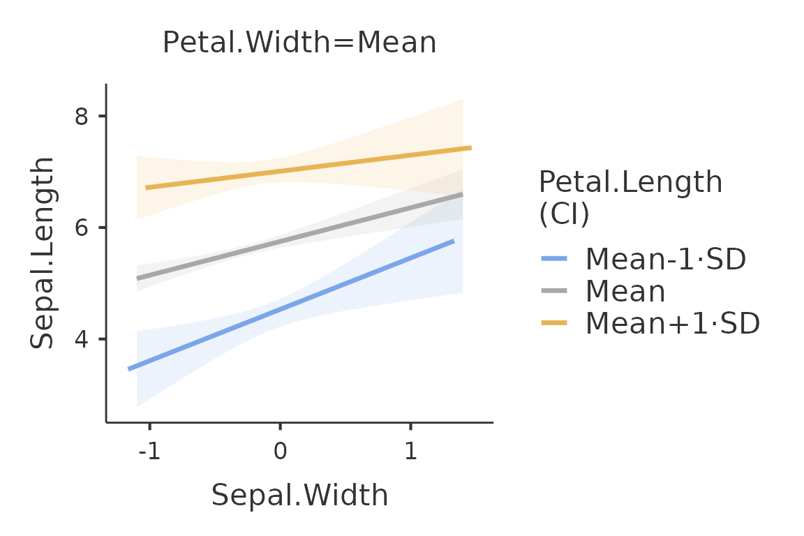
plot(mod,formula = ~Sepal.Width:Petal.Length)

Because the moderator variable Petal.Length is a continuous variable, the function plots the independent variable effect at three different levels of the moderator. By default, the three levels are the mean, the mean plus one standard deviation and the mean minus one standard deviation. The conditioning values can be changed with the option covs_conditioning. The option accepts mean_sd (default) and percent, for 25th,50th, and 75th percentiles.

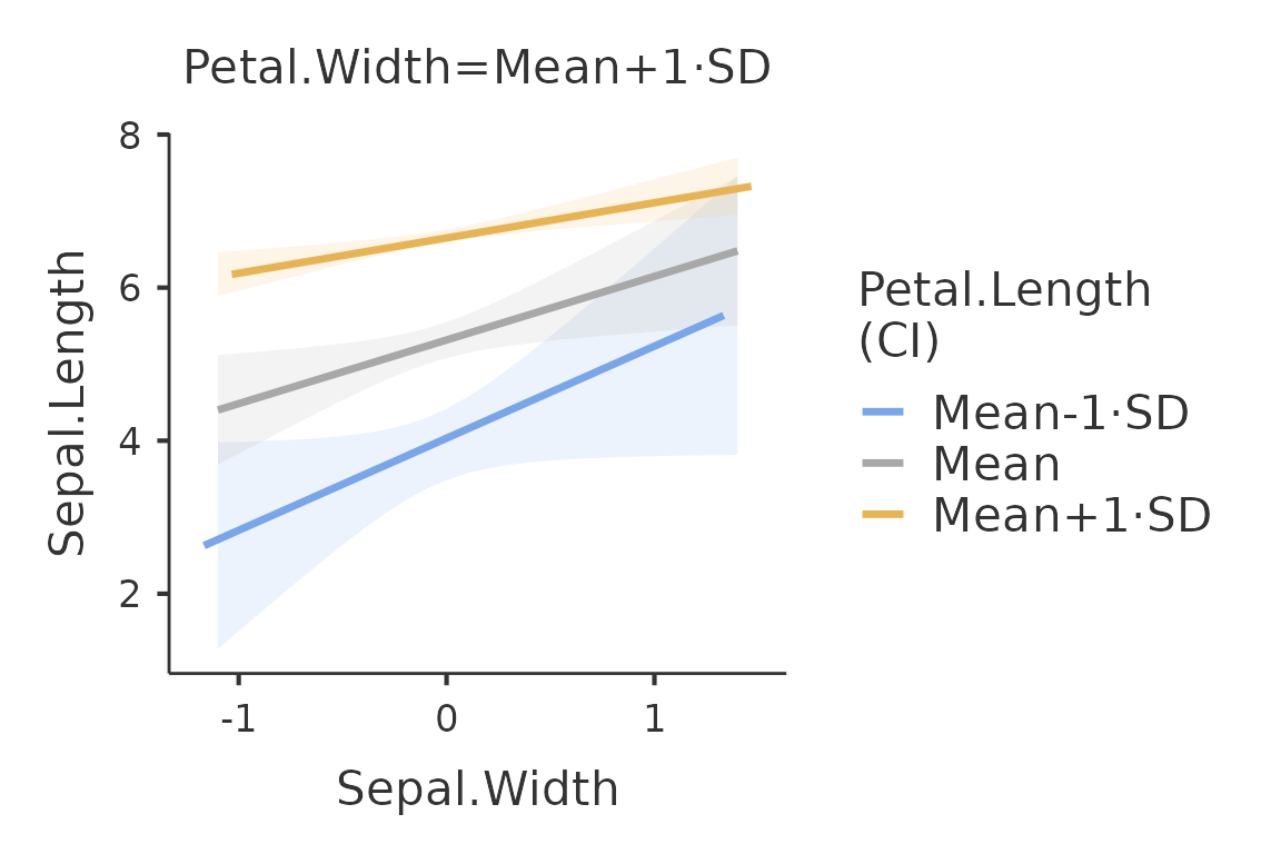
plot(mod,formula = ~Sepal.Width:Petal.Length, covs_conditioning="percent")

Three-way plots

A three-way plot produces one plot for each level of the last moderator, in this case three plots.

plots<-plot(mod,formula = ~Sepal.Width:Petal.Length:Petal.Width)
garbage<-lapply(plots,print)

Because the formula is expanded, one can obtain all main effects and interactions plots in one call by passing formula=~Sepal.Width*Petal.Length*Petal.Width

Factors

When the X-axis variable is a factor, a plot of means is produced.

mod2<-gamlj_lm(formula=Sepal.Length~Species,  data=iris)
plot(mod2,formula=~Species)

Character options

Alternatively, the function accepts characters options. The three options relevant here are:

plot_x defining the variable in the X-axis
plot_z defining the variable whose levels define the way the effect of the variable in the X-axis is broken down (the moderator)
plot_by defining the variable whose levels define the way the two-way interaction is broken down

A two-way plot, for instance, can be obtained as follows:

plot(mod,plot_x="Sepal.Width", plot_z="Petal.Length")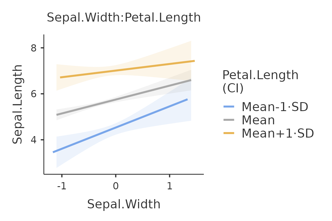

Other options

The function plot accepts any option which is accepted by gaml* functions. The most relevant for producing plots are:

plot_raw (logical) to plot the observed scores along the predicted values
plot_yscale (logical) to set the range of the Y-axis equal to the actual range of the dependent variable (it does not apply to generalized linear models)
plot_xoriginal (logical) to set the scale of the X-axis as the original variable, so not centered or standardized
plot_around to add confidence intervals bars (ci) or error bars se along the predicted values. Default is none.

plot(mod,plot_x="Sepal.Width", plot_z="Petal.Length", plot_raw=T,plot_around="ci")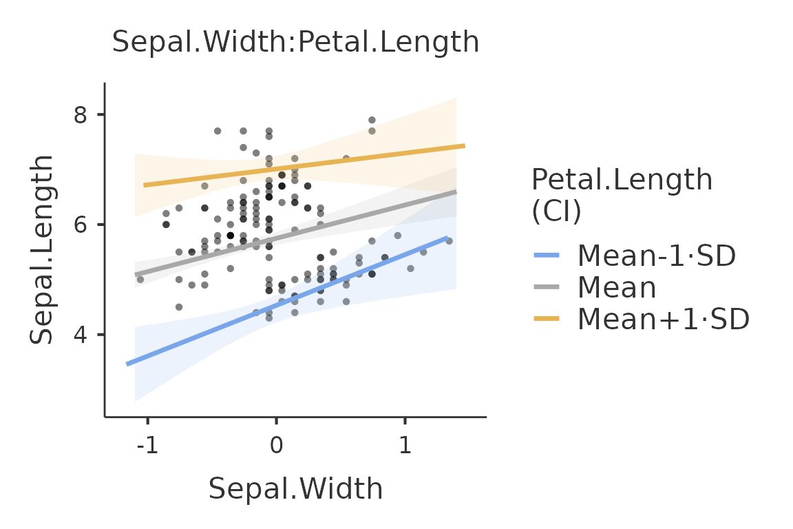

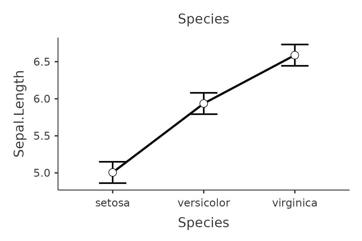
plot(mod2,formula=~Species,plot_raw=T,plot_around="se")

In addition, the plot can be saved in a variable and manipulated as any other ggplot object, for instance to change the theme or add a title.

p<-plot(mod,plot_x="Sepal.Width", plot_z="Petal.Length", plot_raw=T,plot_around="ci")
p+ggplot2::ggtitle("A nice plot")+ggplot2::theme_minimal()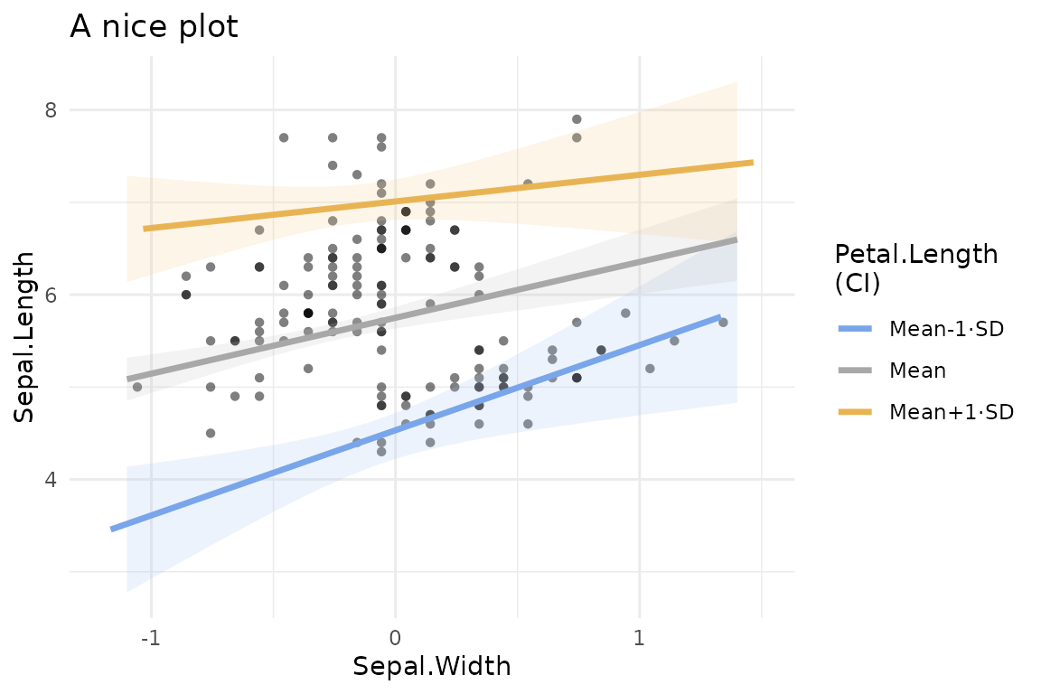

In case of multiple plots produced, the ggplot objects are contained in a list returned by plot().

Other GAMLj functions

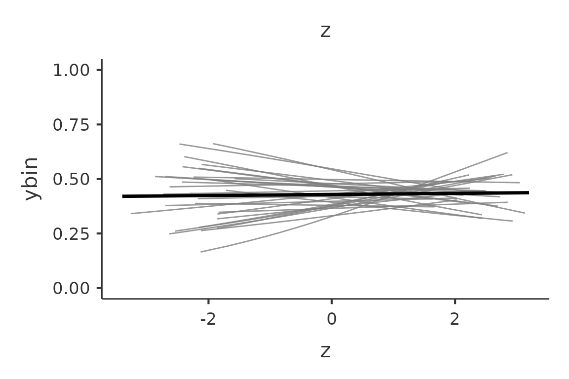
All model functions in GAMLj, (gamlj_lm(),gamlj_glm(),gamlj_mixed() and gamlj_gmixed()), can produce plots using the options and functions described above. Here an example with a generalized (logistic) mixed model in which we plot the fixed and random effects predicted values.

data("clustermanymodels")
clustermanymodels$ybin<-factor(clustermanymodels$ybin)

mod3<-gamlj_gmixed(formula=ybin~z+(1+z|cluster),data=clustermanymodels)

p<-plot(mod3, plot_x = "z",plot_re=T)

Marcello Gallucci

2024-05-16